Machball: a very simple tutorial
This is a simple tutorial on how to use and how to make the most of Machball. It assumes that you have a Python distribution with numpy (which is one of Machball’s dependencies), matplotlib, and Machball installed.
Let’s start by importing matplotlib and numpy:
import matplotlib.pyplot as pt
import numpy as np
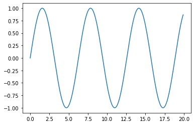
These packages will allow us to work with arrays and matrices as well as to plot the results:
x = np.arange(0,20,0.1)
y = np.sin(x)
pt.plot(x,y)
Defining an ALD process in Machball
Machball defines an ideal ALD process using the ALDIdeal class. It
implements a first order irreversible Langmuir kinetics. Key parameters
are the precursor pressure (in Pa), molecular mass (in amu or
grams/mole), the bare or initial sticking probability (the reactivity of
a precursor molecule towards an available surface site), the temperature
of the process (in K) and the average area of a surface site (in square
meters).
Defining process parameters
We can start by defining some of these parameters:
p = 10
M = 150
beta = 1e-2
T = 473
The average area of a surface site is perhaps the less intuitive of the parameters. However, Machball provides two functions that can be used to calculate this value from the growth per cycle or the mass per cycle.
from machball.utils import sitearea, sitearea_fromqcm
If we look at the documentation of these two functions:
- machball.utils.sitearea(M, density, gpc, nmol=1)
Average area of a surface site
Calculate the average area of a surface site
- Parameters:
M (float) – Molecular mass in atomic mass units
density (float) – Density of the film, in g/cm3
gpc (float) – Growth per cycle, in Angstroms
nmol (int, optional (default 1)) – Number of precursor molecules per unit formula of the solid
- Returns:
Average area of a surface site in sq. meters
- Return type:
float
- machball.utils.sitearea_fromqcm(M, mpc, nmol=1)
Average area of a surface site
Calculate the average area of a surface site from qcm data
- Parameters:
M (float) – Molecular mass in atomic mass units
mpc (float) – Mass per cycle in ng/cm2
nmol (int, optional (default 1)) – Number of precursor molecules per unit formula of the solid
- Returns:
Average area of a surface site in sq. meters
- Return type:
float
These functions help establish a connection between experimental observables and the average area of a surface site. Let’s use 35 ng/cm2 as the mass gain per cycle and the molar mass of Al2O3:
sitearea_fromqcm(102, 35, 2)
Yields:
2.4196991981781087e-19
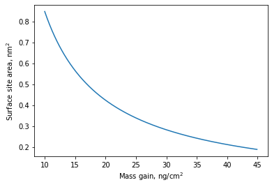
Let’s plot the value of the site area for alumina for a range of mass gain per cycle:
mgain = np.arange(10,45,0.1)
areas = 1e18*sitearea_fromqcm(102, mgain, 2) # Convert to square Angstrom
pt.plot(mgain, areas)
pt.xlabel(r"Mass gain, ng/cm$^2$")
pt.ylabel(r"Surface site area, nm$^2$")
So let’s define a value of s0:
s0 = 20e-20
Working widh ALDIdeal
Let’s import ALDIdeal and define our ALD chemistry:
from machball import ALDIdeal

ald = ALDIdeal(beta, M, T, p, s0, betarec=0)
The first thing we can do is to use the dose method to calculate the
effect of a dose:
ald.dose(0.02) # dose time in seconds
This yields:
0.9809029825287979
The returned value is the fractional coverage after the dose. It is important to remember that, at this point, doses are not accumulative yet. If you repeat the same dose, you will obtain the same value:
ald.dose(0.02)
0.9809029825287979
This is something that will be changed in the next version, to be able to monitor the effect of multiple microdoses
ALDIdeal also has a method for directly calculating the saturation
curve:
times, cov = ald.saturation()
This method returns a list of times and saturation coverages. Let’s plot them:
pt.plot(1e3*times,cov)
pt.xlabel("Dose time, ms")
pt.ylabel("Fractional surface coverage")

We can save the saturation profile to a file using save_saturation
from machball.utils import save_saturation
save_saturation("mysaturation.dat", times, cov)
The default is to save it as a space-delimited file. If instead, you
want to save it as a comma separated value, we need to specify the
csv flag:
save_saturation("mysaturation.csv", times, cov, csv=True)
In both cases the output can be imported pretty much anywhere.
mysaturation.csv can be directly read by any spreadsheet software,
should you use such unholy creatures.
Simulating ballistic transport inside nanostructures
The first step is to define a nanostructure. For this tutorial, we are going to focus on circular vias, which are pre-defined in Machball. However, Machball allows for the simulation of ballistic transport in arbitrary geometries as long as the view factors are provided.
We first need to import and create our nanostructure:
from machball.ballistic import Via
Via discretizes a circular via in a number of equally sized segments
plus the bottom. In order to instantiate a specific via, we need to pass
the aspect ratio, defined as the depth/diameter ratio, and the number of
vertical segments:
st = Via(100, 200)
We can now use the same interface as we used for exploring the evolution of surface coverage on a flat surface. First, we can look at the result of a specific dose:
cov = ald.dose(0.5, st)
The difference with the flat case is that we are passing the
nanostructura as an argument to the dose method of our ALDIdeal
object that we created before.
If we directly plot the output we see the coverage for all the different elements:
pt.plot(cov)
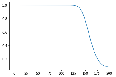
It is important to note, though, that in the output of dose also
contains the coverage in the bottom of the feature. In fact, if we look
at the length of cov:
len(cov)
Yields the following value:
201
cov has 201 elements whereas in the definition of our via we specified
200 vertical segments. The coverage at the bottom is stored in the last
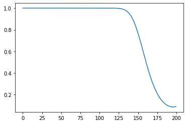
element of the array. Therefore, if we want to plot as a function of
depth, we need to leave that element out:
cov_wall = cov[:-1] # This creates a slice of the array which leaves the last element out
pt.plot(cov_wall)
Like in the flat case, we can also directly calculate the saturation profile. This will give us a sequence of coverage profiles as a function of time:
times2, covs2 = ald.saturation(st, endcov=0.95, verbose=False)
covs2 is a 2D array. If we look at its shape:
covs2.shape
The returned value is:
(97, 201)
We see that each row represents a coverage profile for a given time.
Using slices we can plot specific times:
pt.plot(covs2[10,:-1], label=("%6.4f s" % times2[10]))
pt.plot(covs2[20,:-1], label=("%6.4f s" % times2[20]))
pt.plot(covs2[50,:-1], label=("%6.4f s" % times2[50]))
pt.legend()
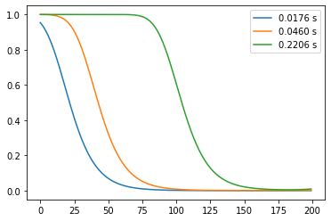
Note that, as before, we have used :-1 to keep just the sidewall
regions of our via. We can also view the 2D array as an image:
pt.imshow(covs2[:,:-1])
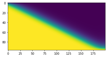
However, it is important to note that the times are not linearly spaced, since Machball uses an adaptive timestep to evolve the fractional coverage with time:
times2
Returns the following array of times:
array([0.00116806, 0.0023257 , 0.00375969, 0.00518084, 0.00659071,
       0.00826952, 0.00993597, 0.01159172, 0.01351175, 0.01542096,
       0.01759161, 0.01975197, 0.02217196, 0.02458257, 0.02725171,
       0.02991249, 0.03283113, 0.0360067 , 0.03917478, 0.04259959,
       0.04601785, 0.04969265, 0.05362351, 0.05754852, 0.06172949,
       0.06590523, 0.07033684, 0.07502397, 0.07970633, 0.08464415,
       0.08957763, 0.09476648, 0.09995134, 0.10539149, 0.11108671,
       0.1167782 , 0.1227247 , 0.12866773, 0.1348657 , 0.14131846,
       0.14776794, 0.15447215, 0.16117329, 0.16812911, 0.17508203,
       0.18228958, 0.18975165, 0.19721095, 0.20492472, 0.21263587,
       0.22060146, 0.22882137, 0.23703878, 0.24551048, 0.25397979,
       0.26270337, 0.27142466, 0.28040019, 0.28962988, 0.29885736,
       0.30833898, 0.31781848, 0.32755208, 0.33728365, 0.3472693 ,
       0.35750897, 0.36774667, 0.37823836, 0.38872815, 0.39947192,
       0.41046959, 0.42146543, 0.43271516, 0.44396312, 0.45546495,
       0.46696506, 0.47871902, 0.49072678, 0.50273287, 0.51499273,
       0.52725095, 0.53976293, 0.5522733 , 0.56503739, 0.57805512,
       0.59107124, 0.60434093, 0.6178641 , 0.63138553, 0.64516024,
       0.65918803, 0.67346856, 0.68800135, 0.70304037, 0.71858358,
       0.73538971, 0.75166171])
We can also plot the average surface coverage as a function of time
pt.plot(times2, np.mean(covs2,axis=1))
pt.xlabel("Dose time (s)")
pt.ylabel("Average surface coverage")

The resulting profiles has the parabolic shape that is expected from a transport-limited process.
Finally, we can export the coverage profiles and the times to a file:
from machball.utils import save_saturationprofile
save_saturationprofile("via100.dat", times2, covs2)
Next steps
This tutorial just went over some of the more basic features of Machball. There are other capabilities we didn’t go through that are fully documented, though not easily accessible. These include the ability to work with other types of eatures, to compare with constant reaction probability processes, and to expand the range of processes to incoporate surface recombination and soft-saturating reactions.